
This section covers works related to Dynamic Time Warping for time series.
Note. In tslearn, such time series would be represented as arrays of
respective
shapes (n, p) and (m, p) and DTW can be computed using the following code:
from tslearn.metrics import dtw, dtw_path

dtw_score = dtw(x, x_prime)
# Or, if the path is also
# an important information:
path, score = dtw_path(x, x_prime)
Dynamic Time Warping (DTW) (Sakoe & Chiba, 1978) is a similarity measure between time series. Consider two time series $\mathbf{x}$ and $\mathbf{x}^\prime$ of respective lengths $n$ and $m$. Here, all elements $x_i$ and $x^\prime_j$ are assumed to lie in the same $p$-dimensional space and the exact timestamps at which observations occur are disregarded: only their ordering matters.
Optimization Problem
In the following, a path $\pi$ of length $K$ is a sequence of $K$ index pairs $\left((i_0, j_0), \dots , (i_{K-1}, j_{K-1})\right)$.
DTW between $\mathbf{x}$ and $\mathbf{x}^\prime$ is formulated as the following optimization problem:
\begin{equation} DTW(\mathbf{x}, \mathbf{x}^\prime) = \min_{\pi \in \mathcal{A}(\mathbf{x}, \mathbf{x}^\prime)} \sqrt{ \sum_{(i, j) \in \pi} d(x_i, x^\prime_j)^2 } \label{eq:dtw} \end{equation}where $\mathcal{A}(\mathbf{x}, \mathbf{x}^\prime)$ is the set of all admissible paths, i.e. the set of paths $\pi$ such that:
- $\pi$ is a sequence $[\pi_0, \dots , \pi_{K-1}]$ of index pairs $\pi_k = (i_k, j_k)$ with $0 \leq i_k < n$ and $0 \leq j_k < m$
- $\pi_0 = (0, 0)$ and $\pi_{K-1} = (n - 1, m - 1)$
for all $k > 0$ , $\pi_k = (i_k, j_k)$ is related to $\pi_{k-1} = (i_{k-1}, j_{k-1})$ as follows:
- $i_{k-1} \leq i_k \leq i_{k-1} + 1$
- $j_{k-1} \leq j_k \leq j_{k-1} + 1$
Here, a path can be seen as a temporal alignment of time series and the optimal path is such that Euclidean distance between aligned (ie. resampled) time series is minimal.
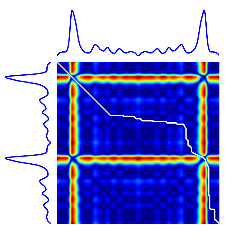
The following image exhibits the DTW path (in white) for a given pair of time series, on top of the cross-similarity matrix that stores $d(x_i, {x}^\prime_j)$ values.
Note. Code to produce such visualization is available in tslearn's
Gallery of
examples.
def dtw(x, x_prime):
  for i in range(n):
    for j in range(m):
      dist = d(x[i], x_prime[j]) ** 2
      if i == 0 and j == 0:
        C[i, j] = dist
      else:
        C[i, j] = dist + min(C[i-1, j] if i > 0
                                       else inf,
                             C[i, j-1] if j > 0
                                       else inf,
                             C[i-1, j-1] if (i > 0 and j > 0)
                                         else inf)

  return sqrt(C[n-1, m-1])
Properties
Dynamic Time Warping holds the following properties:
- $\forall \mathbf{x}, \mathbf{x}^\prime, DTW(\mathbf{x}, \mathbf{x}^\prime) \geq 0$
- $\forall \mathbf{x}, DTW(\mathbf{x}, \mathbf{x}) = 0$
However, mathematically speaking, DTW is not a valid metric since it satisfies neither the triangular inequality nor the identity of indiscernibles.
Setting additional constraints
The set of temporal deformations to which DTW is invariant can be reduced by imposing additional constraints on the set of acceptable paths. Such constraints typically consist in forcing paths to stay close to the diagonal.
%config InlineBackend.figure_format = 'svg'
import matplotlib.pyplot as plt
import numpy

plt.ion()

def clean_plot(title, sz):
    for pos in range(sz):
        plt.plot([-.5, sz - .5], [pos + .5, pos + .5],
                 color='w', linestyle='-', linewidth=3)
        plt.plot([pos + .5, pos + .5], [-.5, sz - .5],
                 color='w', linestyle='-', linewidth=3)
    plt.xticks([])
    plt.yticks([])
    plt.gca().axis("off")
    plt.title(title)
    plt.tight_layout()
The Sakoe-Chiba band is parametrized by a radius $r$ (number of off-diagonal elements to consider, also called warping window size sometimes), as illustrated below:
Note. A typical call to DTW with Sakoe-Chiba band constraint in
tslearn would be:
from tslearn.metrics import dtw
cost = dtw(
  x, x_prime,
  global_constraint="sakoe_chiba",
  sakoe_chiba_radius=3
)
from tslearn.metrics import sakoe_chiba_mask

sz = 10

m = sakoe_chiba_mask(sz, sz, radius=3)
m[m == numpy.inf] = 1.
numpy.fill_diagonal(m, .5)

plt.figure()
plt.imshow(m, cmap="gray")
clean_plot("Sakoe-Chiba mask of radius $r=3$.", sz)
The Itakura parallelogram sets a maximum slope $s$ for alignment paths, which leads to a parallelogram-shaped constraint:
Note. A typical call to DTW with Itakura parallelogram constraint in
tslearn would be:
from tslearn.metrics import dtw
cost = dtw(
  x, x_prime,
  global_constraint="itakura",
  itakura_max_slope=2.
)
from tslearn.metrics import itakura_mask

sz = 10

m = itakura_mask(sz, sz, max_slope=2.)
m[m == numpy.inf] = 1.
numpy.fill_diagonal(m, .5)

plt.figure()
plt.imshow(m, cmap="gray")
clean_plot("Itakura parallelogram mask of maximum slope $s=2$.", sz)