Convolutional Neural Networks#
Convolutional Neural Networks (aka ConvNets) are designed to take advantage of the structure in the data. In this chapter, we will discuss two flavours of ConvNets: we will start with the monodimensional case and see how ConvNets with 1D convolutions can be helpful to process time series and we will then introduce the 2D case that is especially useful to process image data.
ConvNets for time series#
Convolutional neural networks for time series rely on the 1D convolution operator that, given a time series \(\mathbf{x}\) and a filter \(\mathbf{f}\), computes an activation map as:
where the filter \(\mathbf{f}\) is of length \((2L + 1)\).
The following code illustrates this notion using a Gaussian filter:
Show code cell content
%config InlineBackend.figure_format = 'svg'
%matplotlib inline
import matplotlib.pyplot as plt
from notebook_utils import prepare_notebook_graphics
prepare_notebook_graphics()

import numpy as np

def random_walk(size):
    rnd = np.random.randn(size) * .1
    ts = rnd
    for t in range(1, size):
        ts[t] += ts[t - 1]
    return ts

np.random.seed(0)
x = random_walk(size=50)
f = np.exp(- np.linspace(-2, 2, num=5) ** 2 / 2)
f /= f.sum()

plt.figure()
plt.plot(x, label='raw time series')
plt.plot(np.correlate(x, f, mode='same'),
         label='activation map (gaussian smoothed time series)')
plt.legend();

Convolutional neural networks are made of convolution blocks whose parameters are the coefficients of the filters they embed (hence filters are not fixed a priori as in the example above but rather learned). These convolution blocks are translation equivariant, which means that a (temporal) shift in their input results in the same temporal shift in the output:
Show code cell source
from IPython.display import HTML
from celluloid import Camera

f = np.zeros((12, ))
f[:4] = -1.
f[4:8] = 1.
f[8:] = -1.

length = 60

fig = plt.figure()
camera = Camera(fig)

for pos in list(range(5, 35)) + list(range(35, 5, -1)):
    x = np.zeros((100, ))
    x[pos:pos+length] = np.sin(np.linspace(0, 2 * np.pi, num=length))

    act = np.correlate(x, f, mode='same')

    plt.subplot(2, 1, 1)
    plt.plot(x, 'b-')
    plt.title("Input time series")
    fig2 = plt.subplot(2, 1, 2)
    plt.plot(act, 'r-')
    plt.title("Activation map")

    axes2 = fig.add_axes([.15, .35, 0.2, 0.1]) # renvoie un objet Axes
    axes2.plot(f, 'k-')
    axes2.set_xticks([])
    axes2.set_title("Filter")

    plt.tight_layout()
    camera.snap()

anim = camera.animate()
plt.close()

HTML(anim.to_jshtml())
/tmp/ipykernel_5101/368849627.py:32: UserWarning: This figure includes Axes that are not compatible with tight_layout, so results might be incorrect.
  plt.tight_layout()
/tmp/ipykernel_5101/368849627.py:23: MatplotlibDeprecationWarning: Auto-removal of overlapping axes is deprecated since 3.6 and will be removed two minor releases later; explicitly call ax.remove() as needed.
  fig2 = plt.subplot(2, 1, 2)
/tmp/ipykernel_5101/368849627.py:32: UserWarning: The figure layout has changed to tight
  plt.tight_layout()
Convolutional models are known to perform very well in computer vision applications, using moderate amounts of parameters compared to fully connected ones (of course, counter-examples exist, and the term “moderate” is especially vague).
Most standard time series architectures that rely on convolutional blocks are straight-forward adaptations of models from the computer vision community ([Le Guennec et al., 2016] relies on an old-fashioned alternance between convolution and pooling layers, while more recent works rely on residual connections and inception modules [Fawaz et al., 2020]). These basic blocks (convolution, pooling, residual layers) are discussed in more details in the next Section.
These time series classification models (and more) are presented and benchmarked in [Fawaz et al., 2019] that we advise the interested reader to refer to for more details.
Convolutional neural networks for images#
We now turn our focus to the 2D case, in which our convolution filters will not slide on a single axis as in the time series case but rather on the two dimensions (width and height) of an image.
Images and convolutions#
As seen below, an image is a pixel grid, and each pixel has an intensity value in each of the image channels. Color images are typically made of 3 channels (Red, Green and Blue here).
Show code cell source
from matplotlib import image

image = image.imread('../data/cat.jpg')
image_r = image.copy()
image_g = image.copy()
image_b = image.copy()
image_r[:, :, 1:] = 0.
image_g[:, :, 0] = 0.
image_g[:, :, -1] = 0.
image_b[:, :, :-1] = 0.

plt.figure(figsize=(20, 8))
plt.subplot(2, 3, 2)
plt.imshow(image)
plt.title("An RGB image")
plt.axis("off")

for i, (img, color) in enumerate(zip([image_r, image_g, image_b],
                                     ["Red", "Green", "Blue"])):
    plt.subplot(2, 3, i + 4)
    plt.imshow(img)
    plt.title(f"{color} channel")
    plt.axis("off")

Fig. 2 An image and its 3 channels (Red, Green and Blue intensity, from left to right).#
The output of a convolution on an image \(\mathbf{x}\) is a new image, whose pixel values can be computed as:
In other words, the output image pixels are computed as the dot product between a convolution filter (which is a tensor of shape \((2K + 1, 2L + 1, c)\)) and the image patch centered at the given position.
Let us, for example, consider the following 9x9 convolution filter:
Show code cell source
sz = 9

filter = np.exp(-(((np.arange(sz) - (sz - 1) // 2) ** 2).reshape((-1, 1)) + ((np.arange(sz) - (sz - 1) // 2) ** 2).reshape((1, -1))) / 100.)
filter_3d = np.zeros((sz, sz, 3))
filter_3d[:] = filter.reshape((sz, sz, 1))


plt.figure()
plt.imshow(filter_3d)
plt.axis("off");

Then the output of the convolution of the cat image above with this filter is the following greyscale (ie. single channel) image:
Show code cell source
from scipy.signal import convolve2d

convoluted_signal = np.zeros(image.shape[:-1])
for c in range(3):
    convoluted_signal += convolve2d(image[:, :, c], filter_3d[:, :, c], mode="same", boundary="symm")

plt.figure()
plt.imshow(convoluted_signal, cmap="gray")
plt.axis("off");

One might notice that this image is a blurred version of the original image. This is because we used a Gaussian filter in the process. As for time series, when using convolution operations in neural networks, the contents of the filters will be learnt, rather than set a priori.
CNNs à la LeNet#
In [LeCun et al., 1998], a stack of convolution, pooling and fully connected layers is introduced for an image classification task, more specifically a digit recognition application. The resulting neural network, called LeNet, is depicted below:

Fig. 3 LeNet-5 model#
Convolution layers#
A convolution layer is made of several convolution filters (also called kernels) that operate in parallel on the same input image. Each convolution filter generates an output activation map and all these maps are stacked (in the channel dimension) to form the output of the convolution layer. All filters in a layer share the same width and height. A bias term and an activation function can be used in convolution layers, as in other neural network layers. All in all, the output of a convolution filter is computed as:
where \(c\) denotes the output channel (note that each output channel is associated with a filter \(f^c\)), \(b_c\) is its associated bias term and \(\varphi\) is the activation function to be used.
Tip
In keras, such a layer is implemented using the Conv2D class:
import keras_core as keras
from keras.layers import Conv2D

layer = Conv2D(filters=6, kernel_size=5, padding="valid", activation="relu")
Padding
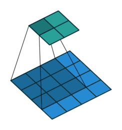
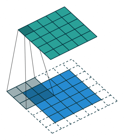
Fig. 4 A visual explanation of padding (source: V. Dumoulin, F. Visin - A guide to convolution arithmetic for deep learning). Left: Without padding, right: With padding.#
When processing an input image, it can be useful to ensure that the output feature map has the same width and height as the input image. This can be achieved by padding the input image with surrounding zeros, as illustrated in Fig. 4 in which the padding area is represented in white.
Pooling layers#
Pooling layers perform a subsampling operation that somehow summarizes the information contained in feature maps in lower resolution maps.
The idea is to compute, for each image patch, an output feature that computes an aggregate of the pixels in the patch. Typical aggregation operators are average (in this case the corresponding layer is called an average pooling layer) or maximum (for max pooling layers) operators. In order to reduce the resolution of the output maps, these aggregates are typically computed on sliding windows that do not overlap, as illustrated below, for a max pooling with a pool size of 2x2:

Such layers were widely used in the early years of convolutional models and are now less and less used as the available amount of computational power grows.
Tip
In keras, pooling layers are implemented through the MaxPool2D and AvgPool2D classes:
from keras.layers import MaxPool2D, AvgPool2D

max_pooling_layer = MaxPool2D(pool_size=2)
average_pooling_layer = AvgPool2D(pool_size=2)
Plugging fully-connected layers at the output#
A stack of convolution and pooling layers outputs a structured activation map (that takes the form of 2d grid with an additional channel dimension). When image classification is targeted, the goal is to output the most probable class for the input image, which is usually performed by a classification head that consists in fully-connected layers.
In order for the classification head to be able to process an activation map, information from this map needs to be transformed into a vector.
This operation is called flattening in keras, and the model corresponding to Fig. 3 can be implemented as:
from keras.models import Sequential
from keras.layers import InputLayer, Conv2D, MaxPool2D, Flatten, Dense

model = Sequential([
    InputLayer(input_shape=(32, 32, 1)),
    Conv2D(filters=6, kernel_size=5, padding="valid", activation="relu"),
    MaxPool2D(pool_size=2),
    Conv2D(filters=16, kernel_size=5, padding="valid", activation="relu"),
    MaxPool2D(pool_size=2),
    Flatten(),
    Dense(120, activation="relu"),
    Dense(84, activation="relu"),
    Dense(10, activation="softmax")
])
model.summary()
Model: "sequential"
_________________________________________________________________
 Layer (type)                Output Shape              Param #
=================================================================
 conv2d (Conv2D)             (None, 28, 28, 6)         156

 max_pooling2d (MaxPooling2  (None, 14, 14, 6)         0
 D)

 conv2d_1 (Conv2D)           (None, 10, 10, 16)        2416

 max_pooling2d_1 (MaxPoolin  (None, 5, 5, 16)          0
 g2D)

 flatten (Flatten)           (None, 400)               0

 dense (Dense)               (None, 120)               48120

 dense_1 (Dense)             (None, 84)                10164

 dense_2 (Dense)             (None, 10)                850

=================================================================
Total params: 61706 (241.04 KB)
Trainable params: 61706 (241.04 KB)
Non-trainable params: 0 (0.00 Byte)
_________________________________________________________________
References#
- FFW+19
Hassan Ismail Fawaz, Germain Forestier, Jonathan Weber, Lhassane Idoumghar, and Pierre-Alain Muller. Deep learning for time series classification: a review. Data Mining and Knowledge Discovery, 33(4):917–963, 2019.
- FLF+20
Hassan Ismail Fawaz, Benjamin Lucas, Germain Forestier, Charlotte Pelletier, Daniel F Schmidt, Jonathan Weber, Geoffrey I Webb, Lhassane Idoumghar, Pierre-Alain Muller, and François Petitjean. Inceptiontime: finding alexnet for time series classification. Data Mining and Knowledge Discovery, 34(6):1936–1962, 2020.
- LGMT16
Arthur Le Guennec, Simon Malinowski, and Romain Tavenard. Data Augmentation for Time Series Classification using Convolutional Neural Networks. In ECML/PKDD Workshop on Advanced Analytics and Learning on Temporal Data. Riva Del Garda, Italy, September 2016.
- LBBH98
Yann LeCun, Léon Bottou, Yoshua Bengio, and Patrick Haffner. Gradient-based learning applied to document recognition. Proceedings of the IEEE, 86(11):2278–2324, 1998.