Alignment-based Metrics in Machine Learning

When learning from non-aligned time series, being able to use alignment-based metrics at the core of Machine Learning (ML) systems is key.

Classification

Nearest Neighbors

First, the similarity measures presented in this chapter can be used in conjunction with nearest-neighbor classifiers. To do so, it suffices to compute DTW (or any other time-series-specific) between a test time series \(\mathbf{x}\) and all the series from the training set, and then assign a label to \(\mathbf{x}\) based on a voting strategy.

Note however that nearest neighbor searches in standard euclidean spaces are usually fastened by smart indexing strategies that are no longer available when using DTW in place of Euclidean distance. A typical example is the use of triangular inequality to prune the set of candidate neighbors (recall that DTW does not satisfy the triangular inequality).

tslearn tip

To use these metrics for \(k\)-Nearest-Neighbor classification in tslearn, the code is as follows:

knn_clf = KNeighborsTimeSeriesClassifier(n_neighbors=3, metric="dtw")
knn_clf.fit(X_train, y_train)
predicted_labels = knn_clf.predict(X_test)

Global Alignment Kernel

Let us define the Global Alignment Kernel (GAK, [Cuturi et al., 2007]) as:

(13)\[\begin{equation} k_\text{GA}^\gamma(\mathbf{x}, \mathbf{x}^\prime) = \exp{- \frac{\text{soft-}DTW^{\gamma}(\mathbf{x}, \mathbf{x}^\prime)}{\gamma}} \end{equation}\]

Though this kernel is not proved to be positive semi-definite (except in the univariate case [Blondel et al., 2020]), authors claim that, in practice, resulting Gram matrices happen to be psd in most of their experiments, hence allowing this kernel to be used in standard kernel methods, as discussed in the next section. One typical use-case consists in using this kernel in Support Vector Machines for classification. When doing so, resulting support vectors are hence time series, as shown below:

Show code cell source Hide code cell source

%config InlineBackend.figure_format = 'svg'
import matplotlib.pyplot as plt
import warnings
warnings.filterwarnings('ignore')

plt.ion()

import numpy

from tslearn.datasets import CachedDatasets
from tslearn.preprocessing import TimeSeriesScalerMinMax
from tslearn.svm import TimeSeriesSVC

numpy.random.seed(0)
X_train, y_train, X_test, y_test = CachedDatasets().load_dataset("Trace")
X_train = TimeSeriesScalerMinMax().fit_transform(X_train)
X_test = TimeSeriesScalerMinMax().fit_transform(X_test)

clf = TimeSeriesSVC(kernel="gak", gamma=.1)
clf.fit(X_train, y_train)

n_classes = len(set(y_train))

plt.figure(figsize=(6, 6))
support_vectors = clf.support_vectors_
for i, cl in enumerate(set(y_train)):
    plt.subplot(n_classes, 1, i + 1)
    plt.title("Support vectors for class %d" % cl)
    for ts in support_vectors[i]:
        plt.plot(ts.ravel())

plt.tight_layout()

Note that methods presented in this section straight-forwardly extend to regression setups in which the target variable is not a time series itself (for this specific case, refer to our Forecasting section).

Clustering

As shown above in our Alignment-based metrics section, using standard clustering algorithms can cause trouble when dealing with time-shifted time series.

In what follows, we discuss the use of Dynamic Time Warping at the core of \(k\)-means clustering.

The \(k\)-means algorithm repeats the same two steps until convergence:

1. assign all samples to their closest centroid ;

2. update centroids as the barycenters of the samples assigned to their associated cluster.

Step 1 only requires to compute distances. Euclidean distance can hence straight-forwardly be replaced by Dynamic Time Warping in order to get shift invariance. Step 2 requires the ability to compute barycenters.

These modifications allow to run a \(k\)-means algorithm with DTW as the core metric:

from tslearn.clustering import TimeSeriesKMeans
from tslearn.datasets import CachedDatasets
from tslearn.preprocessing import TimeSeriesScalerMeanVariance

seed = 0
numpy.random.seed(seed)

# Below is some data manipulation to make the dataset smaller
X_train, y_train, X_test, y_test = CachedDatasets().load_dataset("Trace")
X_train = X_train[y_train < 4]  # Keep first 3 classes
numpy.random.shuffle(X_train)
# Keep only 50 time series
X_train = TimeSeriesScalerMeanVariance().fit_transform(X_train[:50])
sz = X_train.shape[1]

# DBA-k-means
dba_km = TimeSeriesKMeans(n_clusters=3,
                          metric="dtw",
                          verbose=False,
                          random_state=seed)
y_pred = dba_km.fit_predict(X_train)

plt.figure(figsize=(9, 3))
for yi in range(3):
    plt.subplot(1, 3, 1 + yi)
    for xx in X_train[y_pred == yi]:
        plt.plot(xx.ravel(), "k-", alpha=.2)
    plt.plot(dba_km.cluster_centers_[yi].ravel(), "r-")
    plt.xlim(0, sz)
    plt.ylim(-4, 4)
    plt.text(0.55, 0.85,'Cluster %d' % (yi + 1),
             transform=plt.gca().transAxes)

As a result, clusters gather time series of similar shapes, which is due to the ability of Dynamic Time Warping (DTW) to deal with time shifts, as explained above. Second, cluster centers (aka centroids) are computed as the barycenters with respect to DTW, hence they allow to retrieve a sensible average shape whatever the temporal shifts in the cluster.

Another option to deal with such time shifts is to rely on the kernel trick. Indeed, the kernel \(k\)-means algorithm [Dhillon et al., 2004], that is equivalent to a \(k\)-means that would operate in the Reproducing Kernel Hilbert Space associated to the chosen kernel, can be used in conjunction with Global Alignment Kernel (GAK).

Fig. 4 Kernel \(k\)-means clustering with Global Alignment Kernel. Each subfigure represents series from a given cluster.

A first significant difference (when compared to \(k\)-means) is that cluster centers are never computed explicitly, hence time series assignments to cluster are the only kind of information available once the clustering is performed.

Second, one should note that the clusters generated by kernel-\(k\)-means, while allowing for some time shifts, are still phase dependent (see clusters 2 and 3 that differ in phase rather than in shape). This is because, contrary to DTW, Global Alignment Kernel is not invariant to time shifts, as discussed earlier for the closely related soft-DTW.

Forecasting

As discussed earlier, soft-DTW is differentiable with respect to its inputs. This is especially useful for forecasting tasks in which prediction is to be made for multiple time steps (multi-step ahead forecasting)1. Indeed, in this context, soft-DTW can be used in place of a standard Mean Squared Error (MSE) loss in order to better take time shifts into account.

This is done, for example, in the seminal paper by Cuturi and Blondel [Cuturi and Blondel, 2017]:

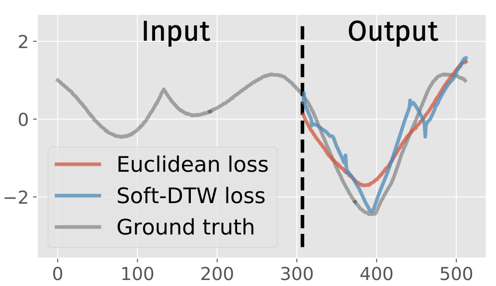
Fig. 5 Using soft-DTW in place of a standard Euclidean loss for forecasting. This Figure is taken from [Cuturi and Blondel, 2017].

An alternative differentiable loss (DILATE) is introduced in [Le Guen and Thome, 2019] that relies on soft-DTW and penalizes de-synchronized alignments. This is done by introducing an additional penalty to the loss to be optimized, which is the dot product between a “soft-mask matrix” \(\Omega\) and the computed soft path matrix \(A_\gamma\), which tends to favor diagonal matches :

(14)\[\begin{equation} \mathcal{L}_\text{reg} = \mathcal{L}_\text{soft-DTW} + \langle \Omega , A_\gamma \rangle . \end{equation}\]

The \(\Omega\) matrix typically looks like:

Show code cell source Hide code cell source

plt.figure()

n = 30
positions = numpy.arange(n) / n
#      ↓ column vector of positions   ↓ row vector of positions
mat = (positions.reshape((-1, 1))   - positions.reshape((1, -1))) ** 2

plt.xticks([])
plt.yticks([])
plt.imshow(mat)
plt.colorbar();

As a result, the DILATE method allows to both better model shape matching than MSE and better localize shapes than soft-DTW:

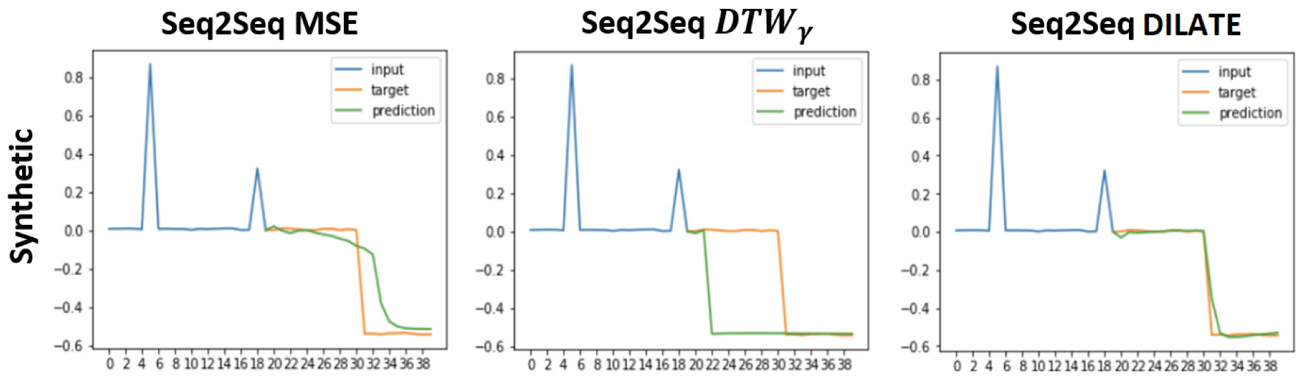
Fig. 6 Comparison between MSE, soft-DTW (denoted \(DTW_\gamma\)) and DILATE as loss functions for forecasting tasks. This Figure is taken from [Le Guen and Thome, 2019].

Conclusion

In this part of the course, we have presented similarity measures for time series that aim to tackle time shift invariance (a.k.a. temporal localization invariance) and their use at the core of various machine learning models.

Dynamic Time Warping is probably the most well-known measures among those presented here. We have shown how to use it in standard classification models as well as for \(k\)-means clustering, in which case a notion of barycenter has to be defined. We have also presented one of its strongest limitations which is its non-differentiability, which has led to the introduction of a soft variant that can hence be used as a loss (for structured prediction settings) in neural networks.

References

BMV20

Mathieu Blondel, Arthur Mensch, and Jean-Philippe Vert. Differentiable divergences between time series. 2020. arXiv:2010.08354.

CB17(1,2)

Marco Cuturi and Mathieu Blondel. Soft-DTW: a differentiable loss function for time-series. In Proceedings of the International Conference on Machine Learning, 894–903. JMLR. org, 2017.

CVBM07

Marco Cuturi, Jean-Philippe Vert, Oystein Birkenes, and Tomoko Matsui. A kernel for time series based on global alignments. In Proceedings of the IEEE International Conference on Acoustics, Speech, and Signal Processing, volume 2, II–413. IEEE, 2007.

DGK04

Inderjit S Dhillon, Yuqiang Guan, and Brian Kulis. Kernel k-means: spectral clustering and normalized cuts. In Proceedings of the ACM SIGKDD International Conference on Knowledge Discovery and Data mining, 551–556. 2004.

LGT19(1,2)

Vincent Le Guen and Nicolas Thome. Shape and time distortion loss for training deep time series forecasting models. In Neural Information Processing Systems, 4189–4201. 2019.

---

1

This problem is an instance of a more general class of problems known as structured prediction problems, in which the target variable (to be predicted) has a specific structure (time series, graph, etc.).